TidyTuesday (22): Cocktails
knitr::opts_chunk$set(fig.width=12, fig.height=8) Initialize
library("tidyverse")
library("scales")
library("patchwork")
library("tidytuesdayR")
# load the data
tuesdata <- tidytuesdayR::tt_load('2020-05-26')
cocktails <- tuesdata$cocktailsEDA
Number of Ingredients
cocktails %>%
  group_by(drink) %>% mutate(mx = max(ingredient_number)) %>%
  group_by(mx) %>% tally() %>%
  ggplot(aes(x = as.factor(mx), y = n)) +
  geom_col(aes(fill = n)) +
  geom_label(aes(label = n), fill = "#c7673e", size = 4) +
  ggthemes::theme_fivethirtyeight() +
  ggthemes::scale_fill_continuous_tableau(palette = "Blue") +
  guides(fill = FALSE) +
  labs(title = "Number of Ingredients")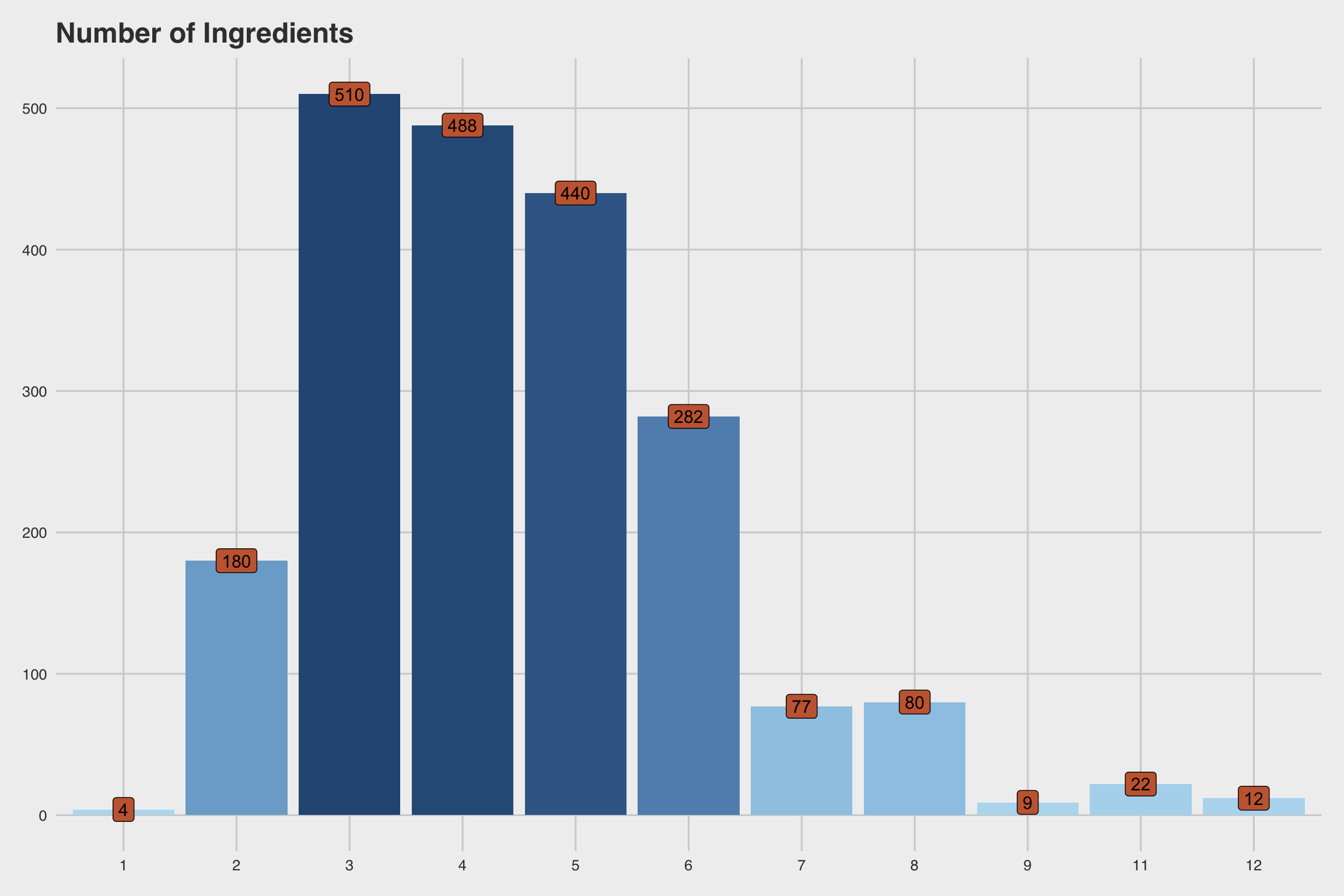
Counts
cocktail_bar_plot <- function(y, title){
  cocktails %>%
    group_by({{y}}) %>% summarize(n = n()) %>%
    arrange(desc(n)) %>% slice(1:12) %>%
    mutate(pct = n/sum(n)) %>%
    ggplot(aes(x = fct_reorder({{y}},n), y = n)) +
    geom_col(aes(fill = n)) +
    geom_label(aes(label = percent(pct, accuracy = 1)), fill = "#c7673e") +
    coord_flip() +
    ggthemes::theme_fivethirtyeight() +
    ggthemes::scale_fill_continuous_tableau(palette = "Blue") +
    guides(fill = FALSE)+
    labs(title = title)
}

p1 <- cocktail_bar_plot(ingredient,"Ingredients")
p2 <-cocktail_bar_plot(iba,"IBA")
p3 <-cocktail_bar_plot(alcoholic,"Alcoholic")
p4 <-cocktail_bar_plot(category,"Category")
p5 <-cocktail_bar_plot(glass,"Glass")

p1+p3+p4+p5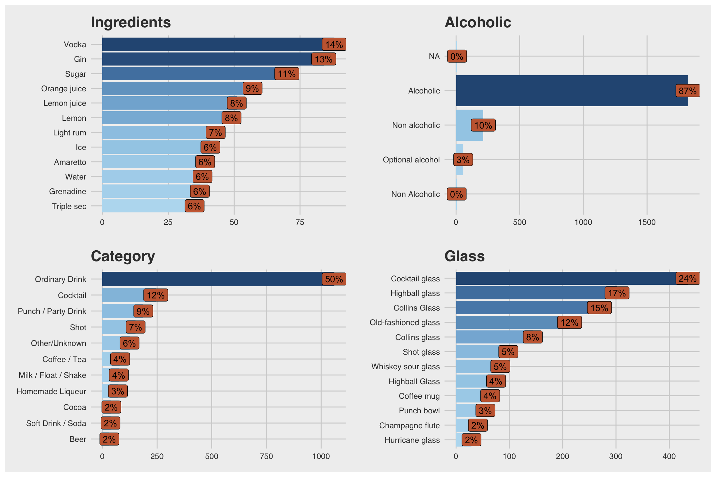
Upset Plot
x<-cocktails %>%
  select(drink,ingredient) %>%
  mutate(b = 1) %>%
  pivot_wider(names_from = ingredient, values_from = b, values_fill = 0, values_fn = length) %>%
  select(-drink) %>%
  as.data.frame()

x[x>1] <- 1

UpSetR::upset(x, nsets = 7,
              main.bar.color = "SteelBlue",
              sets.bar.color = "DarkCyan",
              text.scale = c(rep(1.4, 5), 1),
              order.by = "freq")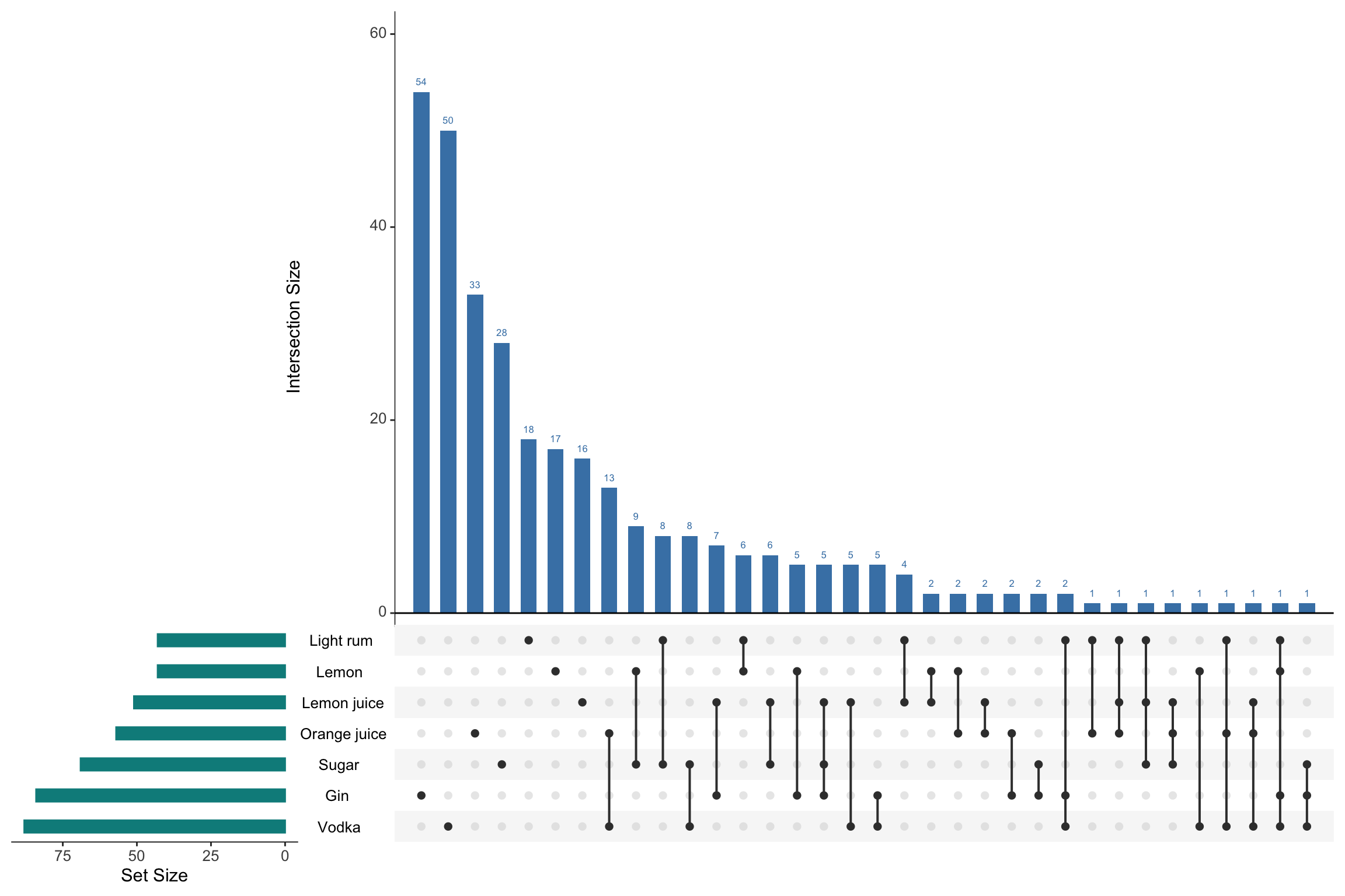
Kyle Thomas
VP, Quantitative Analyst II
I am a quantitative analyst focusing on valuation and marketing.